Examples#
Understanding the Impact of Regularization Parameter Selection#
The following example shows the effects of the selection of the regularization parameter on the estimated coefficients. A simulated signal was generated using a variety of block and spike activation patterns, and adding gaussian noise. The regularization path was solved using the LARS algorithm for both the spike and block models.
import numpy as np
from pySPFM.deconvolution.hrf_generator import HRFMatrix

n_scans = 760
tr = 1

noise_level = 1.5

onsets = np.zeros(n_scans)

hrf_generator = HRFMatrix(te=[0], block=False)
hrf = hrf_generator.generate_hrf(tr=tr, n_scans=n_scans).hrf_

onsets = np.zeros(n_scans)
onsets[20:24] = 1
onsets[50:64] = 1
onsets[67:72] = 1
onsets[101:124] = 1
onsets[133:140] = 1
onsets[311:324] = 1
onsets[372:374] = 1
onsets[420:424] = 1
onsets[450:464] = 1
onsets[467:472] = 1
onsets[501:524] = 1
onsets[550:564] = 1
onsets[567:572] = 1
onsets[601:624] = 1
onsets[660:664] = 1
onsets[701:714] = 1
onsets[730:744] = 1

data_clean = np.dot(hrf, onsets)
data = data_clean + np.random.normal(0, noise_level, data_clean.shape)
data = (data - np.mean(data))/np.mean(data)
data = data/np.sqrt(np.sum(data**2, axis=0))
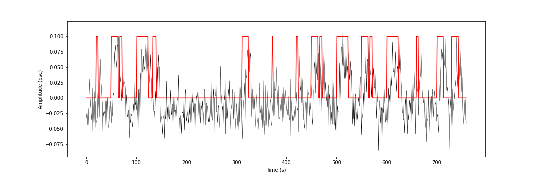
Here is a look at the simulated signal:
Spike model#
Assuming that the data has already been read and normalized to percent signal change, the following code snippet shows how to solve the regularization path using the spike model:
from pySPFM.deconvolution.hrf_generator import HRFMatrix
from pySPFM.deconvolution.lars import solve_regularization_path

n_scans = 760
tr = 1
hrf_generator = HRFMatrix(te=[0], block=False)
hrf = hrf_generator.generate_hrf(tr=tr, n_scans=n_scans).hrf_

_, lambda_opt, coef_path, lambdas = solve_regularization_path(hrf, data, n_scans)
The estimates of activity-inducing signal for each value of \(\lambda\) in the regularization path are shown on the plot below[1]. Move the slider to see the effect of the regularization parameter on the estimated coefficients.
You can see how the maximum value of \(\lambda\) returns no estimates, while the lowest value overfits the data. The estimated spikes capture the moment the BOLD response starts. Remember that the value of \(\lambda\) has to be selected carefully to obtain a good balance between bias and variance. You can do so by selecting the estimates that minimize the Bayesian Information Criterion (BIC) or the Akaike Information Criterion (AIC) for example.
Block model#
The same can be done for the block model:
from pySPFM.deconvolution.hrf_generator import HRFMatrix
from pySPFM.deconvolution.lars import solve_regularization_path

n_scans = 760
tr = 1
hrf_generator = HRFMatrix(te=[0], block=True)
hrf = hrf_generator.generate_hrf(tr=tr, n_scans=n_scans).hrf_

_, lambda_opt, coef_path, lambdas = solve_regularization_path(hrf, data, n_scans)
Remember that with the block model, the sparsity constraint is applied to the derivative of the activity-inducing signal, which allows us to obtain the innovation signal. These estimates of the innovation signal are visible on the plot below. Move the slider to see the effect of the regularization parameter on the estimated coefficients.
You can see that the innovation signal captures the instances where the BOLD response starts and ends. Once again, the value of \(\lambda\) has to be selected carefully to obtain a good balance between bias and variance.
What do AUC time series look like?#
To avoid having to select the regularization parameter manually, we can use the Stability Selection method. This method works by subsampling the data multiple times and solving the regularization path for each subsample. You can think of it as a cross-validation approach. This process provides a snapshot of which time points are selected more frequently. For each value of lambda, the method calculates the probability that every time point has a non-zero coefficient, based on how often it is selected across all runs. These probability curves (one per time point) are then used to calculate the area under the curve (AUC). The AUC serves as a proxy for how likely a time point is to have a non-zero coefficient across all possible lambdas, and therefore to be truly non-zero. The following code snippet shows how to use the Stability Selection method:
from pySPFM.deconvolution.hrf_generator import HRFMatrix
from pySPFM.deconvolution.stability_selection import stability_selection
n_lambdas = 100
n_surrogates = 100

hrf_generator = HRFMatrix(te=[0], block=False)
hrf = hrf_generator.generate_hrf(tr=tr, n_scans=n_scans).hrf_

auc = stability_selection(hrf, data, n_lambdas, n_surrogates)
The AUC time series for the spike model is shown below:
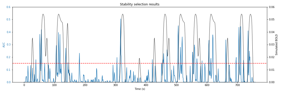
By definition, the AUC time series cannot have zero values. However, that will only happen if the entire space of the regularization path is explored; i.e., if all the regularization parameters are considered. This means that we still have to apply a threshold to the AUC time series to obtain the final estimates. One way to do this is to select a region of the brain where you do not expect to see any activity, like the deep white matter. Assuming you have run stability selection throughout the brain, you can calculate the histogram of AUC values in the deep white matter (you can just erode the white matter mask to make it deep enough). You can then use the 95th percentile (or 99th, depending on how strict or sparse you want your estimates to be) of this histogram as a threshold throughout the brain.
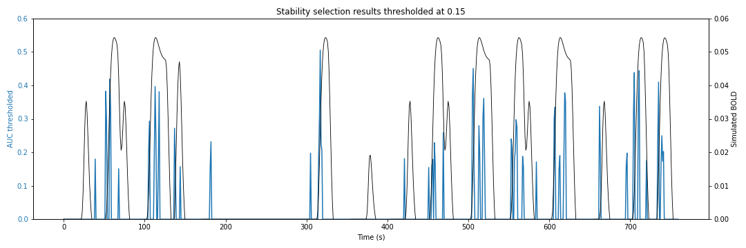
Here is what the thresholded AUC time series would look like if we thresholded the AUC time series above with a 0.15 threshold: